Quantum Algorithm to Solve System of Linear Equations and Inequalities

This project presents a quantum algorithm to solve systems of linear equations and inequalities with the following restrictions:

• The possible values of the variables are 0,1
• The possible solutions are in the interval: [-v,v], where v is the number of variables

The algorithm is based on the Grover´s algorithm and it is able to show all the possible solutions to the system of equation or inequality and moreover, is able to detect when there is no solution.

In the fist step you will see a brief introduction to the Grover´s algorithm.

In the second step the three parts of the Grover´s algorithm have been configurated to solve the following system of equations with two variables and one solution:

x + y = 2

y = 1

In the third step the quantum algorithm has been configurated to solve the following system of one equation and one inequality with two variables and two solutions:

x + y = 1

x + y < 2

In the fourth step the quantum algorithm has been configurated to solve the following system of equations with two variables without solution:

x + 1 = 1

x + y = 2

In the fifth step the quantum algorithm has been configurated to solve the following system of equations with three variables and three solutions:

y + z > 1

x = 1

I have used Qiskit to implement the algorithm and all the python code used can be downloaded from here

The algorithm works with any number of variables and with any number of equations or inequalities.

In all the above examples, you will realize the advantage of the quantum algorithm to solve this kind of systems versus classical algorithms.

I hope it be useful.

You have likely heard that one of the many advantages a quantum computer has over a classical computer is its superior speed searching databases. Grover's algorithm demonstrates this capability. This algorithm can speed up an unstructured search problem quadratically, but its uses extend beyond that; it can serve as a general trick or subroutine to obtain quadratic run time improvements for a variety of other algorithms. This is called the amplitude amplification trick.

Grover's algorithm consists of three main algorithms steps:

1. State preparation. The state preparation is where we create the search space, which is all possible cases the answer could take
2. The oracle. The oracle is what marks the correct answer, or answers we are looking for
3. The diffusion operator magnifies these answers so they can stand out and be measured at the end of the algorithm.

(extract it from Qiskit course)

The system of equations to solve is the following

x + y = 2

y = 1

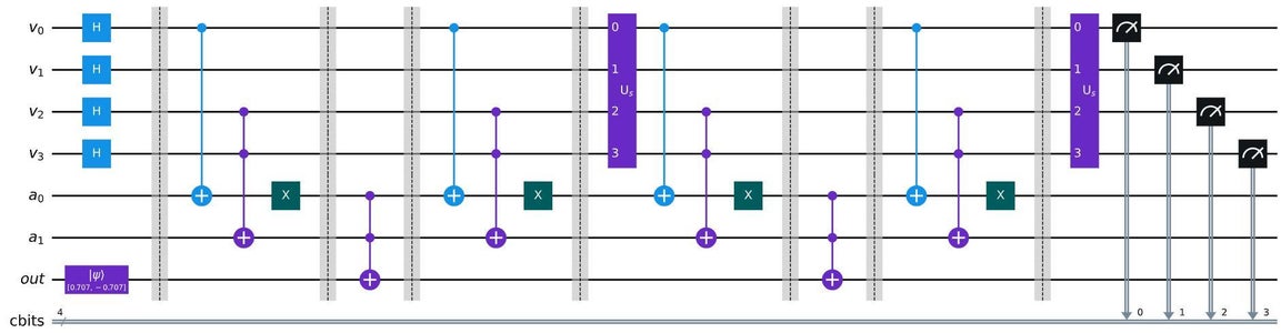
State preparation

This example is a system of two equation with two variables (x,y), so we will need four qubits (v):

• v0 and v1 for x and y variables in the first equation
• v2 and v3 for x and y variables in the second equation

We will need two auxiliary qubits (a0, a1) and one output qubit (ouput)

The algorithm begins applying the Hadamard-gate to 'v0','v1','v2','v3', qubits creating a uniform superposition state and initializing 'output' qubit to the state |->

Please, see the pictures

The oracle

The oracle is what marks the correct answer, or answers we are looking for.

def oracle():
  # Compute auxiliaries
  ### to compute the solutions for x+y=2
  qc.mct([[var_qubits[0]],var_qubits[1]],aux_qubits[0])

  ### to compute the solutions for y=1
  qc.cx(var_qubits[3], aux_qubits[1])

  # Flip 'out' qubit if all auxiliary qubits are satisfied
  qc.barrier()
  qc.mct(aux_qubits, out_qubit)
  qc.barrier()

  # Uncompute clauses to reset auxiliary-checking qubits to 0

  ### to uncompute the solutions for x+y=2
  qc.mct([[var_qubits[0]],var_qubits[1]],aux_qubits[0])

  ### to uncompute the solutions for y=1
  qc.cx(var_qubits[3], aux_qubits[1])

The diffusion operator

It magnifies these answers so they can stand out and be measured at the end of the algorithm.

The diffusion operator is always the same and it has been implemented by Quiskit

def diffuser(nqubits):
  qc = QuantumCircuit(nqubits)
  # Apply transformation |s> -> |00..0> (H-gates)
  for qubit in range(nqubits):
    qc.h(qubit)
  # Apply transformation |00..0> -> |11..1> (X-gates)
  for qubit in range(nqubits):
    qc.x(qubit)
  # Do multi-controlled-Z gate
  qc.h(nqubits-1)
  qc.mct(list(range(nqubits-1)), nqubits-1) # multi-controlled-toffoli
  qc.h(nqubits-1)
  # Apply transformation |11..1> -> |00..0>
  for qubit in range(nqubits):
    qc.x(qubit)
  # Apply transformation |00..0> -> |s>
  for qubit in range(nqubits):
    qc.h(qubit)
  # We will return the diffuser as a gate
  U_s = qc.to_gate()
  U_s.name = "U$_s$"
  return U_s

The solution

Because the size of the search space is 16 and the number of answers expected are 2, we will need two iterarions of the algorithm to solve the system

The solutions will be the bit strings with a much higher probability of measurement than any of the others with the following restrictions:

• v0 = v2 = x
• v1 = v3 = y

In this case the only bit string that matches these restrictions is '1111' (v3 v2 v1 v0) (please, see the picture)

So, we can say that this system of equations has one solution: x=1 ; y=1

You can download the whole python code from here

The system to solve is the following

x + y = 1

x + y < 2

State preparation

This example is a system of one equation and one inequality with two variables (x,y), so we will need four qubits (v):

• v0 and v1 for x and y variables for the equation
• v2 and v3 for x and y variables for the inequality

We will need two auxiliary qubits (a0, a1) and one output qubit (ouput)

The algorithm begins applying the Hadamard-gate to 'v0','v1','v2','v3', qubits creating a uniform superposition state and initializing 'output' qubit to the state |->

Please, see the pictures

The oracle

The oracle is what marks the correct answer, or answers we are looking for.

def oracle():
  # Compute auxiliaries
  ### to compute the solutions for x+y=1
  qc.cx(var_qubits[0], aux_qubits[0])
  qc.cx(var_qubits[1], aux_qubits[0])


  ### to compute the solutions for x+y<2
  qc.mct([[var_qubits[2]],[var_qubits[3]]],aux_qubits[1])
  qc.x(aux_qubits[1])

  # Flip 'out' qubit if all auxiliary qubits are satisfied
  qc.barrier()
  qc.mct(aux_qubits, out_qubit)
  qc.barrier()

  # Uncompute clauses to reset auxiliary-checking qubits to 0

  ### to uncompute the solutions for x+y=1
  qc.cx(var_qubits[0], aux_qubits[0])
  qc.cx(var_qubits[1], aux_qubits[0])

  ### to uncompute the solutions for x+y<2
  qc.mct([[var_qubits[2]],[var_qubits[3]]],aux_qubits[1])
  qc.x(aux_qubits[1])

The diffusion operator

It magnifies these answers so they can stand out and be measured at the end of the algorithm.

The diffusion operator is always the same and it has been implemented by Quiskit (see step #2)

The solution

Because the size of the search space is 16 and the number of answers expected are 6, we will need only one iterarion of the algorithm to solve the system

The solutions will be the bit strings with a much higher probability of measurement than any of the others with the following restrictions:

• v0 = v2 = x
• v1 = v3 = y

In this case two bit strings match these restrictions: '0101' and '1010' (v3 v2 v1 v0) (please, see the picture)

So, we can say that this system of equations has two solutions:

1. x=1 ; y=0
2. x=0 ; y=1

You can download the whole python code from here

The system of equations to solve is the following

x + 1 = 1

x + y = 2

State preparation

This example is a system of two equation with two variables (x,y), so we will need four qubits (v):

• v0 and v1 for x and y variables in the first equation
• v2 and v3 for x and y variables in the second equation

We will need two auxiliary qubits (a0, a1) and one output qubit (ouput)

The algorithm begins applying the Hadamard-gate to 'v0','v1','v2','v3', qubits creating a uniform superposition state and initializing 'output' qubit to the state |->

Please, see the pictures

The oracle

The oracle is what marks the correct answer, or answers we are looking for.

def oracle():
  # Compute auxiliaries
  ### to compute the solutions for x+1=1
  qc.cx(var_qubits[0], aux_qubits[0])
  qc.x(aux_qubits[0])

  ### to compute the solutions for x+y=2
  qc.mct([[var_qubits[2]],[var_qubits[3]]],aux_qubits[1])

  # Flip 'out' qubit if all auxiliary qubits are satisfied
  qc.barrier()
  qc.mct(aux_qubits, out_qubit)
  qc.barrier()

  # Uncompute clauses to reset auxiliary-checking qubits to 0

  ### to uncompute the solutions for x+1=1
  qc.cx(var_qubits[0], aux_qubits[0])
  qc.x(aux_qubits[0])

  ### to uncompute the solutions for x+y=2
  qc.mct([[var_qubits[2]],[var_qubits[3]]],aux_qubits[1])

The diffusion operator

It magnifies these answers so they can stand out and be measured at the end of the algorithm.

The diffusion operator is always the same and it has been implemented by Quiskit (see step #2)

The solution

Because the size of the search space is 16 and the number of answers expected are 6, we will need only one iterarion of the algorithm to solve the system.

The solutions will be the bit strings with a much higher probability of measurement than any of the others with the following restrictions:

• v0 = v2 = x
• v1 = v3 = y

In this case there is not any bit string that matches the restrictions. (please, see the picture)

So, we can say that the system of equations has no solution.

You can download the whole python code from here

The system to solve is the following

x = 1

y + z < 2

State preparation

This example is a system with one equation and one inequality with three variables (x,y,z), so we will need six qubits (v):

• v0, v1, v2 for x, y, z variables in the equation
• v3, v4, v5 for x, y, z variables in the inequality

We will need two auxiliary qubits (a0, a1) and one output qubit (ouput)

The algorithm begins applying the Hadamard-gate to 'v0','v1','v2','v3','v4','v5' qubits creating a uniform superposition state and initializing 'output' qubit to the state |->

Please, see the pictures

The oracle

The oracle is what marks the correct answer, or answers we are looking for.

def oracle():
  # Compute auxiliaries
  ### to compute the solutions for x=1
  qc.cx(var_qubits[0], aux_qubits[0])


  ### to compute the solutions for y+z<2
  qc.mct([[var_qubits[4]],[var_qubits[5]]],aux_qubits[1])
  qc.x(aux_qubits[1])

  # Flip 'out' qubit if all auxiliary qubits are satisfied
  qc.barrier()
  qc.mct(aux_qubits, out_qubit)
  qc.barrier()

  # Uncompute clauses to reset auxiliary-checking qubits to 0

  ### to uncompute the solutions for x=1
  qc.cx(var_qubits[0], aux_qubits[0])

  ### to uncompute the solutions for y+z<2
  qc.mct([[var_qubits[4]],[var_qubits[5]]],aux_qubits[1])
  qc.x(aux_qubits[1])

The diffusion operator

It magnifies these answers so they can stand out and be measured at the end of the algorithm.

The diffusion operator is always the same and it has been implemented by Quiskit (see step #2)

The solution

Because the size of the search space is 64 and the number of answers expected are 25, we will need only one iterarion of the algorithm to solve the system

The solutions will be the bit strings with a much higher probability of measurement than any of the others with the following restrictions:

• v0 = v3 = x
• v1 = v4 = y
• v2 = v6 = z

In this case three bit strings match these restrictions: '011011' ; '001001' ; '101101' (v5 v4 v3 v2 v1 v0) (please, see the picture)

So, we can say that this system has three solutions:

1. x=1 ; y=1 ; z=0
2. x=1 ; y=0 ; z=0
3. x=1; y=0 ; z=1

In this case, you can see clearly the advantage of the quantum algorithm, because in only one iteration is able to calculate the solutions of the system.

You can download the whole python code from here